Trading Articles
Using The Euro To Trade Gold By Anthony Trongone

Reaching a critical price in one commodity often triggers an emotional response by investors in other commodities. Here’s a look at the relationship between a leading variable and a lagging one. Reaching a critical price in one commodity often triggers an emotional response by investors in other commodities. Market participants quickly react to these price disruptions, and their response eventually trickles down to less-active momentum players. Once enough market participants begin jumping aboard, this pattern — with its basis in market sentiment — establishes a foothold.
This article focuses on the intraday activity of two commodity contracts: the leading variable and lagging variable, the first of which drives the price of the second. In order to demonstrate how these two variables function, I will use the euro, the official currency of the European Union (EU), as the contributory (leading) variable, and the gold futures contract as the response (lagging) variable. The euro (EC) trades on the GLOBEX, using the US dollar as its currency. It has a multiplier of 125,000 with increments of 0.0001 ($12.50), whereas the gold futures contract (GC) trades on the NYMEX and has a contract size of $100 per troy ounce with a multiplier of 10. I ran this analysis by downloading the numbers for the continuous contracts [6E #F/GC #F] directly from Interactive Data.
ECONOMIC BACKGROUND
The fear of another “Greek-style” fiscal crisis spreading to other EU countries puts additional pressure on the euro, mostly over concerns about the solvency of its members. In reaction, central banks began turning off the tap in an effort to stem the flow of easy financing. This sudden shift to such a stringent monetary policy exerted a negative impact on its currency. The rapid depreciation of the euro (red line in Figure 1) can be seen in the double-axis line chart comparing the two futures contracts.
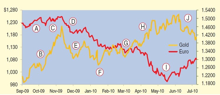
Seizing the opportunity presented by the euro’s continuous decline, many investors chose to play a forex combination such as being long sterling but shorting the European currency. In this instance, however, we are focusing on a less-obvious combination. In Figure 1, the performance of the euro from 8:30 am to 10:00 am is applied to forecast the price of the gold futures contract between 10:00 am to 12 noon:
- With the euro holding above $1.4600 (10 am prices),
- The GC contract rallied strongly.
- This currency contract spent the autumn holding at around $1.5000, but upon further attempts to rise above this price, it met continuous resistance.
- Due to its inability to rise, the contract fell sharply below support ($1.4600) before turning sideways.
- With this currency moving sideways, the price of the yellow metal took to the upside but fell back.
- In sympathy with a falling euro, the gold futures contract broke down to $1,050. After losing $53, it ran back up, eventually trading sideways, as gold bugs waited for currency traders to make their move.
- The euro was able to stabilize at $1.3400, but the anticipation of a deteriorating fiscal crisis brought it down below support, sinking heavily to a closing price of $1.1947.
- Reacting to this meltdown, gold bugs went on a buying spree, pushing the currency above $1,250.
- The euro barely held above its January 1999 introduction price of 1€ = 1.1800 USD. Under $1.2000, buyers found this currency attractive, pushing its price upward. With this movement, momentum buyers began resurfacing, lifting its price back toward earlier support.
- Soon after the recovery of the euro was under way, the price of the precious metal took an inverse path.
STARTING THE ANALYSIS
For comparison purposes here, results are given for two different time frames in Figure 2. The separation occurs when the blue (gold futures) dots finally rise above the red (euro) dots. Before the intersection occurs, the pre-crisis (before the green circle) has two price breakdowns as well as two resting points (trades sideways). The post-crisis analysis (after the green circle) begins on April 5, 2010, when the yellow metal finally lifts above the euro.
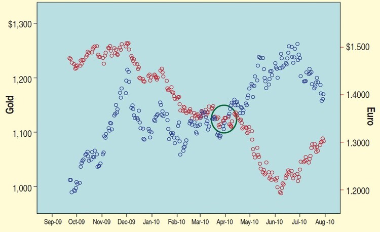
I started the analysis on April 5, 2010, because this was when the two variables went in opposite directions. The green circle indicated when gold broke above its counterpart. A good place to start trading this system is when this currency breaks below support or falls below $1.40, but I take the liberty of starting this analysis after gold finally overtakes the euro.
When attempting to play this system, we are often late arriving to the party. As a result, the post-analysis occurs after the euro begins breaking down prior to its final descent. In this case, there may be an earlier connection between two variables (two commodities or a commodity with a market index or stocks within a business sector), so it may be best to wait until you confirm the connection between the two variables before putting your money on the table or taking a more aggressive position.
LEADING INDICATOR
Early detection of a leading indicator is not always easy, but it often follows a similar pattern. This indicator passes from sideline to headline news as it eventually becomes common knowledge. With the investment community focusing on every tick, a move in the wrong direction can cause panic but trigger investment opportunity. Since these reactions are prompted by the commodity reaching a certain price, if you run the numbers and discover what its turning point is, you will be able to spot new opportunities as they arise.
When you run your analysis, compare the leading variable with the response variable. Are they going in a similar or inverse direction? Remember, you cannot assess the price of the two variables within the same time span. Your analysis of the contributory variable must be before the response variable. In this study, I am using the results of the EC futures contract from 8:30 to 10:00 am; I apply this information to forecast how my response variable will trade from 10:00 am until 12 noon.
Suggested Books and Courses About Trading With Indicators

In playing this leading/ lagging system, traders often make one mistake, and that is expecting the two variables to have an inverse reaction. This is not always the case. As long as the leading variable accurately forecasts the direction of the lagging variable, we can produce favorable results. Although we expect the two variables to go in different directions, more significance often lies in the difference between the two.
The performance of the pre crisis can bring certain results, which are antagonistic to those results in the postcrisis session — that is, given the same price change in the leading indicator, when the pre is positive for the response variable, the post is negative, and when the pre is negative, the post session is positive.
PRE CRISIS
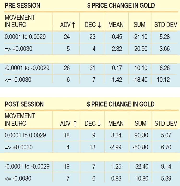
In spite of a rise or fall in this currency, there were conflicting results in the pre session. Gold fell hard after a weak upward (-$21.10) or strong downward change (-$18.40) but ran ahead after a strong uptick ($20.90 in nine days) or a weak downtick ($10.12) in the price of this currency (Figure 3).
POST CRISIS
In the postcrisis session (April 5 to July 31, 2010), an inverse relationship develops (r = -0.857) as these two commodities took turns switching positions, and their prices form the shape of a rhombus. During these 83 trading days, the GC contract rallied $39, from $1,130.40 to $1,169.40 (10 am price). For the system to produce meaningful results, this becomes our basis for comparison. A small rise in the currency pushes the contract up to $90.30 with an 18–9 record, but when the advance was => 0.0030, the GC contract fell $50.80 with 13 declines in 17 plays (Figure 3).
Despite the direction, a small change in the price of the EC contract gave us positive results. A slight weakening of this currency came with an increase in volatility, but a 19–7 record. Most important, however, is the divergence in performance between the pre and post sessions. In the pre session, after a minor currency appreciation, the yellow metal fell in price ($21.20), but in the post session, it chalked up its best performance ($90.30). Again, an opposite reaction took place after a strong currency move to the upside. In this case, the pre session resulted in a $20.90 profit but had some of its biggest losses in the post session, with a loss of $50.80 in 17 plays.
ONGOING PATTERN
Although the results of this study are encouraging, they will not hold forever. The influence these contributory variables have on another variable is fleeting — that is, a leading variable’s effect on the response variable (in this case, the GC commodities contract) will waver in its predictive powers. As in the case of this combination, they may abruptly reverse direction (note the inverse correlation). But it is the knowledge of of how to implement these leading predictor variables that brings significance to this study.
Once you understand how to effectively apply these leading variables, all that remains is to replace them with another variable when it becomes a more significant contributor to the direction of your response variable. The financial papers often highlight the importance of this newcomer in its infancy, and follow-up articles begin appearing, confirming this relationship. The secret to this system’s success comes from early analysis of this new predictive variable as well as early determination of this leading variable before it loses its usefulness as a predictor.
BEST-PERFORMING CATEGORY
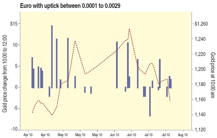
Figure 4 illustrates the best-performing category. When this currency futures contract had a small increase, the GC contract rallied $90.30. A small currency uptick begins with a strong performance, but it falters as the GC contract slides to $1,200. At this point it remains inactive until it begins a steady move to its highest price. The category becomes active again with two strong days, but as this precious metal falls back below $1,200, the system loses some of its shine.
CONCLUSION
These lagging/leading plays come in many combinations. For instance, in early August 2010, there was a commodity/sector play. When the Russian government announced that it was banning exports of wheat, that drove the price of this commodity appreciably higher, to a record price not seen for decades. The fear of a grain shortage caught beer producers by surprise. With the sharp increase in the price of this important ingredient, the stock price of these companies stumbled badly.
When using a contributory variable, there appears to be a counterpoint in which the results completely reverse themselves. For instance, in the post session, a small positive currency change brought a $90 profit, but a strong increase (0.003 * 125000, representing the bottom 15%) took the GC contract down $50.
When breaking your analysis into two separate sessions, it is important to look for an opposite reaction in the movement of the response variable; this occurs when the leading variable undergoes an aberrant price change different from its customary range of activity. Unfortunately, mastery over this leading/lagging variable strategy does not come easily; it takes practice and patience, but the rewards are well worth the effort.
A Master Educator for Interactive Data, Anthony Trongone writes articles on current investment strategies.