Trading Articles
Market Trend And Midas By Andrew Coles and David Hawkins
Here’s an in-depth look at an indicator that is part of Midas, the well-known market data analysis system. In this article, we will look at the formula used to calculate it. The innovative work of the late technical analyst Paul Levine into the application of volume-weighted average price (VWAP) principles to the financial markets has drawn attention in recent years. One result of this work is an indicator many readers will by now be familiar with. Levine called it Midas, an acronym for the market interpretation/data analysis system. The other result of this work is an indicator Levine called the “top-finder/bottom-finder,” the subject of this article.
Outside of Levine’s work, a standard VWAP calculation (the total value of shares traded in a particular stock on a given day divided by the total volume of shares traded in that stock on that same day) is typically used as a benchmark to measure the efficiency of institutional trading. It is also a standard tool in the brokerage industry in that a VWAP execution is a way of earning a trader’s commission. Beyond this, rudimentary VWAP calculations have played a limited role in trading decisions, as in technician Kevin Haggerty’s methodology of establishing whether a stock price has closed above its daily VWAP.
A radical extension of this standard VWAP calculation, however, has resulted in a technical charting indicator capable of fractal market analysis across multiple chart time frames. The Midas indicator on the daily charts generates robust nonlinear support and resistance curves that indicate major trend reversals. Midas has gained a reputation as a powerful indicator of trend exhaustion points in the primary (nine months to two years) and intermediate (six weeks to nine months) trends. However, recent articles have revealed that Levine’s fractal philosophy applies not only to different segments of the daily trend but also to smaller components that can be analyzed on intraday time frames.
Three Main Roles Of The Midas indicator
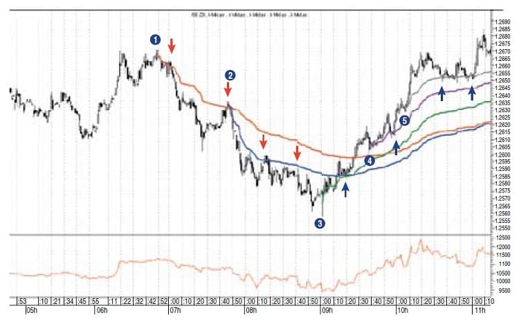
Before moving on, let’s be clear about what the Midas indicator does. Midas is capable of performing three fundamental roles. The first role can be described as a trend-continuity indicator. Figure 1 illustrates this primary role clearly in relation to an uptrend and a downtrend in a V-shaped bottom on a 1m chart of the Euro GlObex December 2008 futures. All ongoing trends, as you may know, have temporary exhaustion points (or pullbacks), and Midas effectively captures the end of these temporary pullbacks.
The second role for Midas is that of an end-of-trend overbought/oversold indicator. This is what Levine referred to as the “hierarchical structure of support and resistance levels.” Levine’s view was that an ongoing trend could support a maximum of four to five Midas curves before it ends.
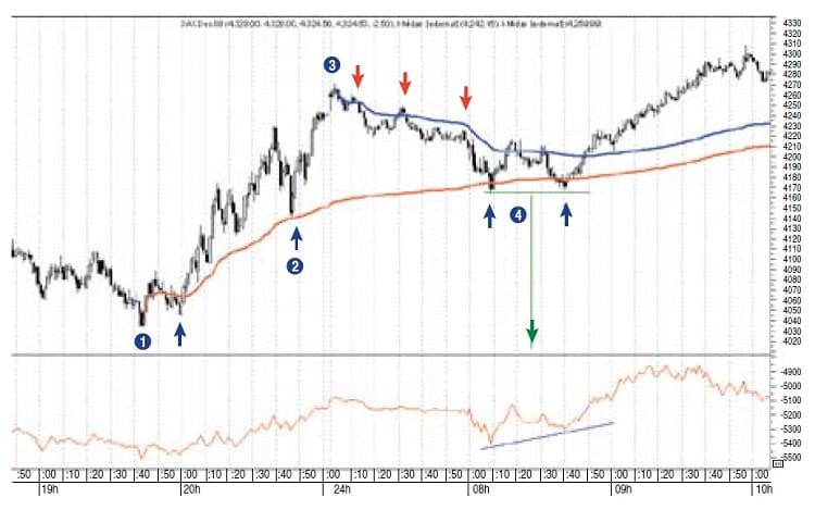
The third role for Midas is that of a reverse-trend target indicator. This is illustrated in Figure 2. Here, an upside trend that has been subject to a Midas curve launched at its inception (point 1) has ended and a new downtrend has begun (point 3). Note the displacement of this early Midas curve from the development of the uptrend (point 2). Because of this, the early Midas curve has now become a price target for the new downtrend. At the double bottom marked by point (4), note the on-balance volume (ObV) diverged positively from price as it made its second bottom. This suggests that the Midas resistance curve would not continue resisting price. At the same time, price reacted powerfully to the displaced Midas support curve, which had become a target for this modest downtrend.
Major Insights Of The Midas Approach
The second role of the Midas indicator carries the first of two major insights that, according to Levine, supplied his overall Vwap approach to the markets. This insight involves the hierarchical structure of support and resistance levels and their predictive nature in terms of Vwap taken over an interval subsequent to a trend reversal point. The second insight is that there often exists an underlying structure that dominates or “guides” the bull or bear move as it develops from the reversal point onward.
Levine believed that this structure was revealed when prices are compared to a new type of theoretical support/resistance curve generated by what he called the top-finder/bottom-finder algorithm, which we will refer to as the TB-F algorithm/indicator, or as its intraday counterpart, TB-Fi. Levine referred to the quantitative laws that give rise to the Midas and the TB-F curves as the scientific component of Midas. He called the engineering aspect the practical trading rules and techniques based on the system. We’ll look at the scientific component of the TB-F algorithm in relation to the original Midas formula while highlighting the core components of TB-F. Then we will teach the basic principles of chart application for TB-F while illustrating its powerful predictive capabilities.
TB-F Algorithm In Relation To Original Midas Formula
The basic equation for the Midas indicator is as follows:
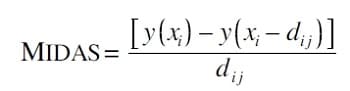
where:
xi = cumulative volume on bar
yi = cumulative average price ((H+L)*0.5) * volume on bar
dij = cumulative volume difference between bars i and j = xi – xj
Here is the equation for the TB-F indicator:
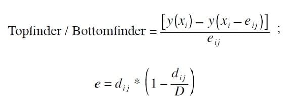
where again:
xi = cumulative volume on bar
yi = cumulative average price ((H+L)*0.5) * volume on bar dij = cumulative volume difference between bars i and j = xi – xj
It should be pointed out that in the programming of the TB-F algorithm, we use the low price when plotting a TB-F support curve and the high price when plotting a TB-F resistance curve instead of Levine’s average price calculation. The former appears to be slightly more accurate.
Critical Role Of D in The TB-F Formula
The primary difference between these two equations is the replacement of d with e, where the effective displacement e is related to the displacement d parabolically through the equation e = d*(1–d/D). D is now a critical new parameter in e which Levine calls the duration of the trend. In fact, D embodies the second major insight of the Midas approach — that is, the underlying structure that guides the bull or bear move as it develops from the reversal point onward. Sometimes Levine wrote about the start of the trend as the launch point of the move and D as a preprogrammed amount of “fuel” which, in this case, is a fixed amount of cumulative volume. As the trend develops, the trajectory follows the curve of the TB-F indicator. When the fixed amount of cumulative volume is burnt out, prices in an uptrend will typically fall back to the most previously active Midas curve (role 3). Occasionally, the trend doesn’t burn up all of the cumulative volume predicted by D; as a result, it ends prematurely. Hence, D should be regarded as a potential outcome and not a guaranteed one. As we see later, when the trend does end, it breaks emphatically through the TB-F curve. Thus, the TB-F algorithm provides a clear indication of a trend’s end even when (occasionally) D is not fully consumed.
Suggested Book: MIDAS Technical Analysis: A VWAP Approach to Trading and Investing in Today’s Markets
In sum, when price reverses and a new trend begins, the expectation is for it to do one of two things: either it will launch in a way required for the application of a TB-F curve, or it will fail to launch, in which case it will merely ride along the Midas curve launched at the same time as the TB-F curve. Occasionally, however, even when TB-F launches successfully, not all of D will be consumed before the trend ends. This is rare, but when it does occur, price will break the TB-F curve, thus signaling the end of the trend. The idea that a trend has a fixed duration should be taken literally, because as we shall see shortly, e goes to zero when d approaches D. This is possible mathematically because D itself represents a fixed volume of whatever is being traded. If TB-F is being applied to the stock market, it would be a fixed volume of shares. When e eventually goes to zero, TB-F will come to a literal stop on the chart. Where and when this occurs is the expected end of the trend. The e component is a complex feature of the TB-F algorithm, so to make it easier for you, it would be helpful if you follow Figure 3.
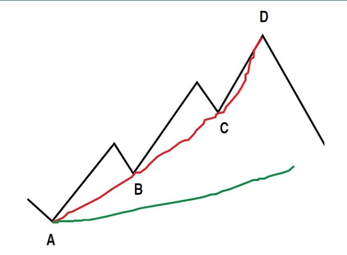
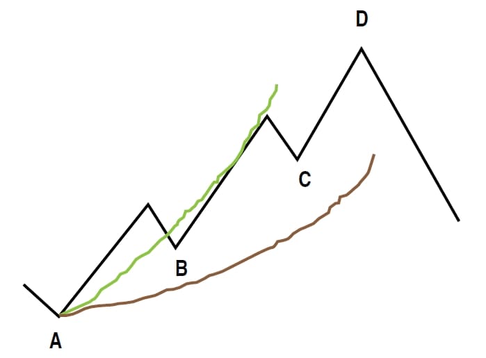
At A, marking the trend starting point, a Midas (green) curve is launched. Note that point B, the end of the first pullback in the trend, does not pull back all the way to the Midas curve. This is a necessary condition of the application of TB-F. In addition, a hypothetical TB-F (red) curve is now launched from point A. We leave the original Midas curve in place because it is now effectively playing role 3 — that is, a reverse-trend-target indicator for the newly established downtrend subsequent to the end of the move predicted by D. So how do we assess how much cumulative volume — the metaphorical fuel for the move — is required for D? The amount of cumulative volume required to predict the end of the move is coextensive with the amount required to “fit” TB-F to the first pullback, which failed to pull all the way back to the recently launched Midas curve (point B). This is an iterative process. If too much cumulative volume is inputted, the TB-F curve will underfit the first pullback; too little, the TB-F curve will overfit it. Figure 4 illustrates an overfit in the pale green line and an underfit in the pale brown.
How can this fitting process be understood mathematically? The answer lies in the relation of D to d in the e part of the new TB-F formula. Bear in mind that as the move progresses from points A to B to C to D, the amount of cumulative volume is increasing. This is d, the cumulative volume displacement in the Midas and the TB-F curves from the launch point to wherever the curve is currently plotting. So if d at point B equals a cumulative volume of, say, 350,000 units and B represents a third of the entire move, the finite amount of cumulative volume for the entire move — that is, D — is 1,050,000 units. This is the fuel required to push the entire move all of the way from point A to its end at point D. So, the Midas curve represents an average price taken over successively longer intervals as the cumulative volume keeps increasing, and the TB-F curve represents an average price taken over successively shorter intervals after the midpoint of the trend as the allotted amount of cumulative volume in D is used up. Levine described this in terms of the launch point of the TB-F algorithm moving forward in time toward the present, finally catching up when the D units of finite cumulative volume have built up subsequent to its launch.
The Parabolic Nature Of E
The parabolic displacement in the TB-F algorithm can be illustrated with the hypothetical example displayed in Figure 5. Assume that at point A the cumulative volume is eight units and at point B it is 15 units. Therefore at B, d = 15 –8 = 7. Now at B, we have assumed that the move is a third through to completion. Therefore, we fit TB-F at a cumulative volume of 21 units. Now, for the sake of this example, let’s assume that from point B to the end of the move to point D, there are exactly 14 closing prices. Thus, at 14 closes between B and D, we have 14 discrete points where we can take a cumulative volume and cumulative price reading.
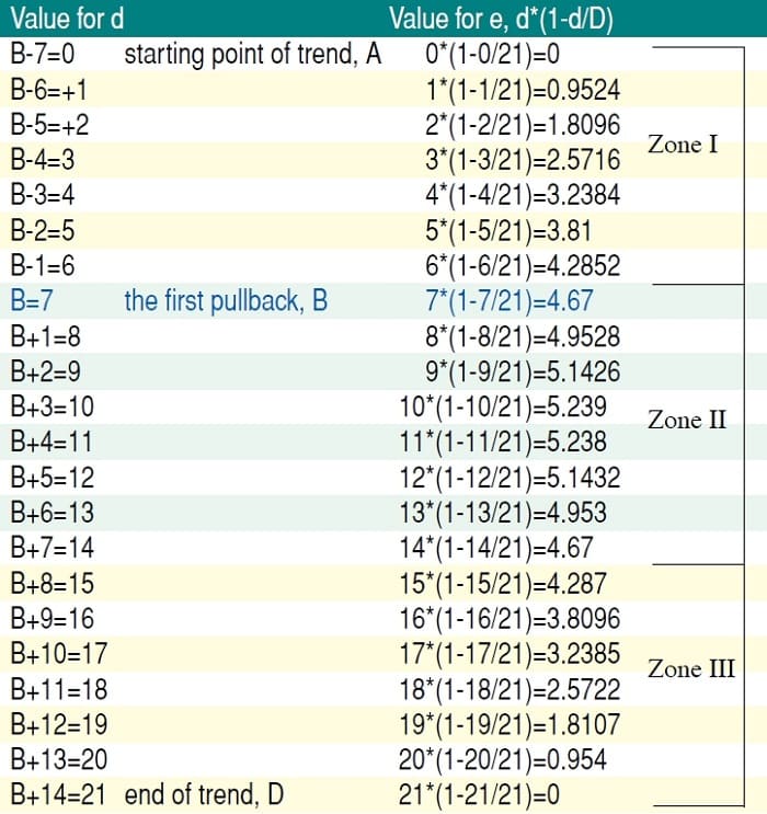
Point B is highlighted in blue and the actual start of the move is B – 7. To keep things simple, let’s assume that each of these 21 closes (including the 7 before B) increases the cumulative volume by one unit. Thus, d will increase accordingly as on the left-hand side, while the corresponding values for e are on the right-hand side.
In zone I, which identifies the trend from the launch (point A) to the first third of the move at point B, e and d are fairly close to each other, with the result that TB-F is not moving that far away from the Midas curve. Bear in mind, however, that it is the failure of price to pull back to the Midas curve, which indicates that we should launch a TB-F curve, since a shorter displacement than d is required to fit to the price pullback at point B. In zone II, we see that the TB-F displacement continues to increase until the halfway point at around B + 4. At this point, price is finding support on the TB-F curve at half of D. In the earlier example, D was 1,050,000 units, so price would be hypothetically finding support at around 525,000 units. In zone III, the displacement is now decreasing rapidly. In fact, toward the end of zone III, for every new unit traded, the averaging interval shortens virtually by one.
Accelerated Price Trend
Levine believed that this dramatic feature of zone III provided the best clue as to what might be going on in a typical trend of the type we have just illustrated. In short, what he concluded can be described in the following terms. Market trends begin when supply is in very little demand. This is the very earliest stage (zone I) in the accumulation phase, which is when traders start entering the market. In this stage there is a rapidly increasing displacement in the TB-F algorithm. The next phase, zone II, is the active trading phase, the strong trend-following portion of the trend dynamic. This is where 70% plus of all trading volume takes place.
Finally, we have the distribution phase, zone III, where the number of offers falls radically and liquidity is vastly reduced. Traders start selling to unusually late newcomers to the end of the trend. Eventually, few buyers are found and zone III quickly turns into the start of a new downtrend as the displacement in D has diminished to zero. What we actually see midway through zone II, however, is that the distribution phase, marked by the start of the diminishing displacement in e, begins a lot earlier than most traders have been aware.
While this does provide a fascinating backdrop to the displacement phenomenon in e, it does not go far enough in capturing the remarkable hidden order that exists in trends. We have already seen that the fixed amount of cumulative volume (the fuel for the entire move) in D is arrived at by fitting the TB-F curve to the first pullback, which doesn’t pull all the way back to the Midas curve. This means there is an essential but hidden relationship between the displacement in the early part of a trend and the amount of cumulative volume used up over the trend’s entire move. If this relationship weren’t there, the TB-F algorithm would not be able to indicate the end of any trend in cumulative volume terms.
Let’s dig deeper. We know that the period between the start of the move and the first pullback is principally the accumulation phase of the trend. In fact, Figure 5 reveals that the displacement keeps on increasing until halfway through zone II. Thus, if we can predict the end of an entire trend in cumulative volume terms from data derived from the accumulation phase of the trend, this means that there must be a much tighter symmetrical relationship between the accumulation phase and the distribution phase than has been recognized. This probably means that the deeper the pullback is into the trend, the more accurate D will be, because most of the cumulative volume data from the accumulation phase will by that time be available. It is not merely, then, that the displacement phenomenon in D captures so precisely the accumulation/trading-zone/distribution phases of each trend. While Levine was surely correct about this, the displacement phenomenon in D also shows the mirror-image symmetry that must exist between the accumulation and distribution phases if the TB-F algorithm is to have any forecasting potency at all.
Interpolation in The TB-F Algorithm
Before seeing TB-F in action, we need to discuss two aspects of the TB-F algorithm that differentiate it from the Midas algorithm. One involves a price interpolation procedure, while the other (as a consequence) requires a high-level programming language that supports looping. It will be beyond the scope of this article to provide instructions on how to interpolate or code the procedure, so we will just explain why interpolation is required. In a standard Midas curve, the height of a point on the curve is calculated by summing the product of price and volume of all the price bars from the current bar back to the launch bar, then dividing that sum by d, the cumulative volume displacement from the launch bar to the present bar. The height of each point on a TB-F curve is similarly calculated, except that the summation does not go all the way back from the present bar to the launch bar. Rather, it goes back along the cumulative volume axis only the number of bars bracketed by e. Subsequently, the summation is divided by e, not d.
The complication comes because e is a continuous variable, whereas each price bar adds a discrete amount of volume along the cumulative volume axis. So in the movement from the present bar back an amount e, the point on the cumulative volume axis arrived at is always between two discrete values — one for a bar of lesser cumulative volume and the next for a bar of greater cumulative volume. Consequently, the next bar to the right of the e point has to be replaced in the summation by a synthetic bar, whose volume is obvious by the location of e and whose price has to be calculated as an interpolation between the price of the original bar and the one preceding it.
A do-loop calculation in the coding of the algorithm is necessary to locate the bar that has to be replaced with a synthetic bar, and then the interpolation between the two prices has to be done in the correct direction, forward in time, which may not be the intuitively obvious thing to do. When the interpolation is done correctly, the resulting curve is smoothly monotonic. To handle this interpolation, it is essential to use a programming language capable of a looping function, because while interpolation itself doesn’t require looping, looping is required to locate the bar. Many languages used by high-end trading platforms do not have this capability. Therefore, it will be necessary to program TB-F in a language such as C++ as an external dll.
UK-based Andrew Coles can be reached at [email protected]. David Hawkins is a private investor, living in Newton, MA.