Trading Articles
Presidential Cycle Seasonality: A Market Timing Study
Mark Vakkur made another significant research contribution by publishing another seminal article in the October 1996. In this rticle, Vakkur combined the optimum months with the optimum presidential cycle years. The results were outstanding; so let’s get right to them.
Vakkur Tests Optimum Months Combined with Optimum Presidential Cycle Years
The election cycle years are:
- Pre-election year: The year before the election year (for example, 1987, 1991, 1995, 1999, and 2003)
- Election year: The year of the election (for example, 1988, 1992, 1996, 2000, and 2004)
- Postelection year: The year after the election year (for example, 1989, 1993, 1997, 2001, and 2005)
- Midterm election year: Two years after the last election year and also prior to the next election year (for example, 1990, 1994, 1998, 2002, and 2006)
Historically, there is a four-year cycle in the stock market encompassing the presidential election years. Usually, the market rises more in the pre-election year than in the election year itself. The election year is the second best of those four years. And in the two years after the election, the market usually does not make much progress. Table 8-1 contains the data from 1950 through 1995 delineating the average monthly returns of the S&P 500 Index in each of the four years of the presidential election cycle, as compiled by Vakkur.
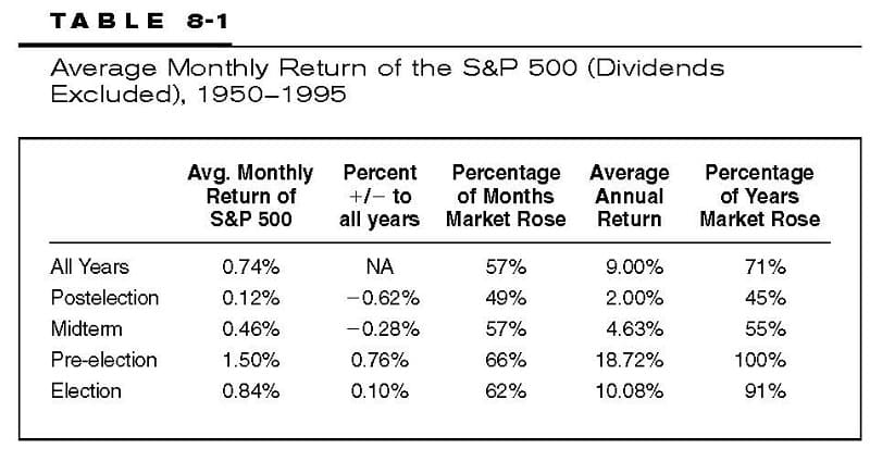
As the table indicates, the pre-election years’ stock market returns are by far superior to any of the other three years of the presidential election cycle. The average annual return since 1950 was 18.72 percent and the market rose every pre-election year. The next best performing year was the election year, with an average annual return of 10.08 percent and a 91 percent success ratio. Conversely, the worst performing presidential cycle year was the postelection year, with an average annual return of only 2 percent and with the markets rising only 45 percent of the time in those years. Next worst performance was the midterm year, which sported an average annual return of a meager 4.63 percent, with a positive market in 55 percent of the years.
Freeburg Tests Presidential Cycle Back to 1886
Nelson Freeburg tested the quadrennial presidential cycle back to 1886 through 2001, to double-check and expand upon the data tested by Vakkur. In the May 31, 2002, issue of FORMULA RESEARCH, Freeburg provided the statistics for the DJIA (refer to Table 8-2).
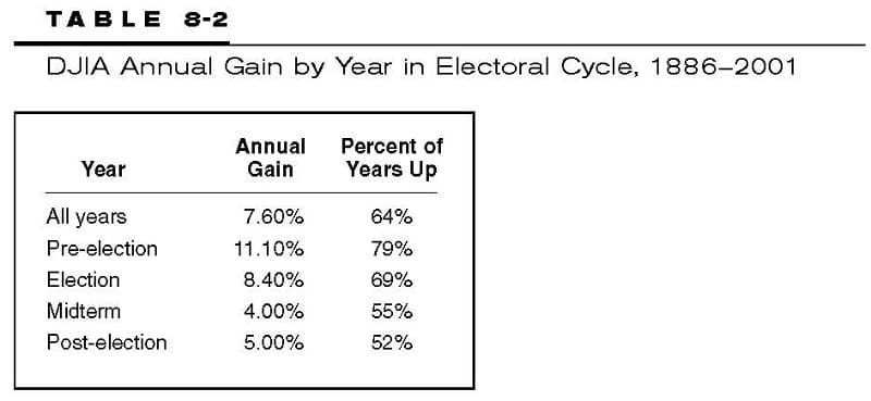
Keep in mind that Vakkur used the S&P 500 Index (without dividends) in calculating his numbers (nominal return), while Freeburg used the DJIA (without dividends), since that index had a much longer price history available. Clearly, there has been a definite bias toward higher stock market returns in the pre-election and election years during the 45 years observed in Vakkur’s analysis, as well as in Freeburg’s more up-to-date and comprehensive analysis.
Vakkur’s Leveraged Strategies Earn Millions
Refer to Table 8-3 to see how an investor fared by taking advantage of Vakkur’s several strategies from 1950 to 1995.3 First, let’s get the lowdown on the returns from buy-and-hold. This often-touted simple no-decision strategy had an average annual return of 8.4 percent that turned a $10,000 initial investment into $372,388 with a 12-month maximum drawdown (or maximum loss of 41.3 percent during the test period). This means that the buy-and-hold investor sat through this loss without flinching. In reality, the average investor would have a hard time doing this.
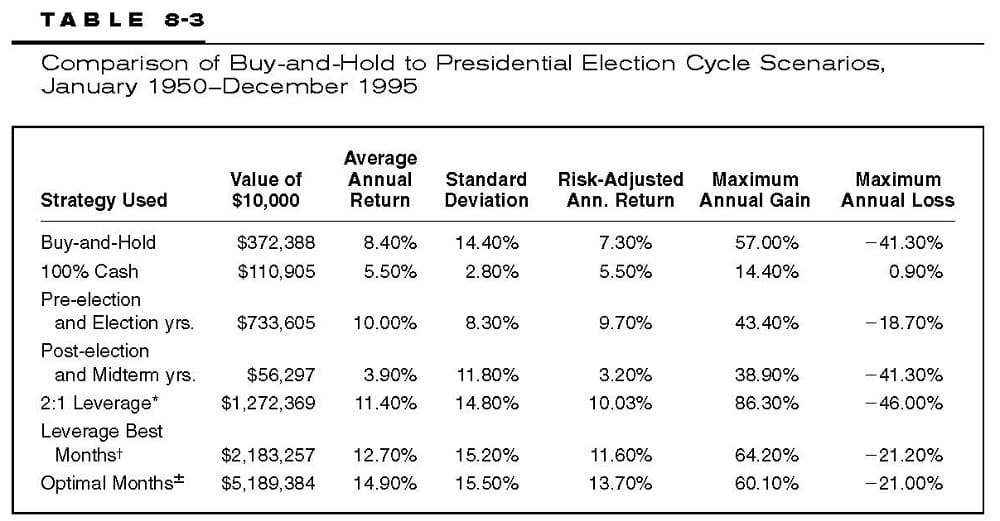
†Leveraged 2:1 (November–April) in the pre-election and election years; 100% invested during these same months in the post-election and mid-term election years, and 100% invested during the May-October period during the same two years. The only time there would be a 100% cash allocation would be in the May-October postelection and mid-term election years.
±Optimal Months:2:1 leverage in pre-election and election years in the following months in those years: January to April, July, November and December; 100% cash in May and September of all 4 years, and June and August of the postelection and midterm election years; and 100% invested in all the other months not mentioned: January to April, July, and October to December in the post-election/midterm years, and June and August in the pre-election years.
Source: Mark, Vakkur, M. D. “Seasonality and the Presidential Election Cycle,” Technical Analysis of Stocks & Commodities, October 1996, vol.14, no.
Now compare those results with the simple strategy of investing only during the best performing two presidential cycle years—the pre-election and election years—and remaining in cash for the other two years. This strategy has an average annual return of 10 percent, which is 1.6 percentage points a year better than buy-and-hold. But over 45 years, that incremental difference resulted in the growth of the $10,000 investment to $733,605, compared to $372,388 for buy-and-hold.
This translates into a 197 percent improvement over buy-and-hold, with a standard deviation of only 8.3 percent versus 14 percent for buy-and-hold, and a maximum 12-month drawdown of only 18.7 percent. So, on all counts, this presidential cycle strategy provided superior results with 50 percent less risk, since you were invested for only two years out of four. In my book, a higher return with less risk is always a win-win strategy.
Advanced Books and Courses on Market Cycles & Timings

You may be curious to see the results of investing only in the worst two performing presidential cycle years—the postelection and midterm election years. As expected, the performance results were much worse than buy-and-hold, with only a 3.9 percent average annual return and the same annual maximum drawdown of 41.3 percent. Even the lowly 100 percent cash portfolio (not investing at all) beat these two years’ performance by generating an average annual return of 5.5 percent with no negative drawdown!
When cash is able to beat buy-and-hold (for the worst two presidential cycle years), you know that you should avoid investing at all. Vakkur tested a number of different strategies to determine their profitability. The first strategy used was with 2:1 leveraging. This strategy used 50 percent margin in the pre-election year, invested funds with no margin in the election year, and was 100 percent in cash for the other two years. As expected, this strategy quadrupled the return of buy and hold.
With an average annual return of 11.4 percent, and an ending balance of $1,272,369, this leveraged strategy provided an additional return of $538,764 over the non-leveraged pre-election and election-year strategy. Using this more aggressive strategy also resulted in more than doubling the maximum annual drawdown (largest loss incurred) to –46 percent from –18.7 percent in the prior strategy. Also, the maximum annual gain jumped about 100 percent, to 86.3 percent from 43.4 percent. And the standard deviation (variability around the 11.4 percent return) rose to 14.8 percent from 8.3 percent.
As Milton Friedman, the Noble Laureate economist, said, “There is no such thing as a free lunch.” And as the saying goes, “no pain, no gain.” As mentioned earlier, risk and reward go hand in hand. Investors who have a higher risk tolerance may want to consider using this leveraged strategy. However, they should use a stop-loss order to minimize the their risk of a large intra-year drawdown and avoid getting clobbered when the market goes against them.
Vakkur tested another leveraged strategy called the Leveraged Best Months (LBM) strategy. Here the best performing months (November to April) of the year were leveraged 2 to 1 (50 percent margin) in the pre-election and election years, 100 percent was invested during these same months in the postelection and midterm election years, and 100 percent was invested during the May–October period during the same two years. The only time that there would be a 100 percent cash allocation would be in the May–October postelection and midterm election years.
This strategy really hit pay dirt, with an annual return of 12.7 percent and total ending principal of $2,183,257. Moreover, both the maximum drawdown and the maximum yearly gain were reduced. And the standard deviation moved up only slightly to 15.2 percent from the previously reviewed 2:1 leveraged strategy of 14.8 percent. On a risk-adjusted basis the LBM strategy is the best tested so far. This strategy was less risky than the 2:1 leveraged strategy while providing an additional $910,888, quite an astounding difference in the bottom line.
Before reviewing another highly profitable leveraged strategy that more than doubled the LBM returns, let’s look at Table 8-4 showing the monthly returns over 45 years in each of the four election cycle years. The best seven months in the pre-election year and election years were January, February, March, April, July, November, and December. The worst months in all the four election cycle years were May and September. Two more worse months occurred in June and August of the postelection and midterm election years. All the other months not mentioned—January, February, March, April, July, October, November, and December in the postelection/midterm years, and June and August in the pre-election years—were considered average months.
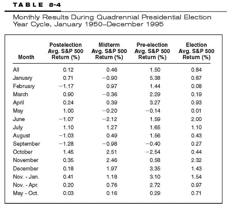
Using this information, Vakkur formulated another highly profitable strategy that he referred to as the “optimal months” strategy. Look at the footnote in Table 8-3, which provides the exact “optimal months” strategy used. That strategy produced an annual return of 14.9 percent, or an astonishing $5,189,384 over the 45 years tested. With only a slightly higher 0.3 percent standard deviation than the LBM strategy and virtually equivalent drawdowns, this strategy added another $3 million to the bottom line. Also, on a risk-adjusted basis, this strategy had the highest annual return of all the strategies illustrated, at 13.7 percent.
Freeburg also tested the strategy of investing in the market (using the DJIA) only in the pre-election and election year from 1886 to 2001, and going into cash in the other two years.4 He found that this strategy resulted in an annual return of 5.9 percent compared to 5.2 percent for buy-and-hold. This 70-basis-point difference, on a$10,000 initial investment, was valued at $8.4 million at the end of the test period, compared to $3.7 million for buy-and-hold. The opposite strategy of investing in the two weakest performing years and going to cash during the two strong years since 1886 has returned 3.6 percent per year, worth $607,000. This is 93 percent less than the optimal strategy.
Freeburg ran additional leveraged tests of the data, using the strongest months in the strongest years, and they confirmed Vakkur’s results. Since Vakkur analyzed the data through 1995, the question is how has the four-year presidential cycle (in particular using the strongest months in the strongest years) performed since then? Freeburg, who updated the data from 1995 through April 2002, found that using Vakkur’s methodology produced an annual gain of 17.4 percent a year compared to 10.7 percent for the buy-and-hold S&P 500 Index. Even since 1886, use of the same methodology has given an annual return of 8.3 percent compared to 5.2 percent for the DJIA.
In conclusion, focusing on the optimal months in the presidential election cycle years really brings home the bacon. This strategy is far superior to just investing during the entire pre-election and election years, with outstanding return and risk parameters.
MIDTERM TO ELECTION YEAR PHENOMENA
Over the years, a number of analysts have scrutinized the presidential cycle years to look for patterns. One very consistent pattern that has been uncovered occurs from the lows of the midterm election cycle year to the highs of the following election year. These results are shown in Table 8-5, which was prepared by the Hays Advisory Group.5 Of the 21 midterm years until the election years, 20 have produced gains. Although the S&P 500 Index gains have ranged from 18.4 percent to 121.9 percent, the average gain has been 56.8 percent. Excluding the only loss of 43.6 percent from 1930 to 1932, the average gain for the period has been 61.8 percent.
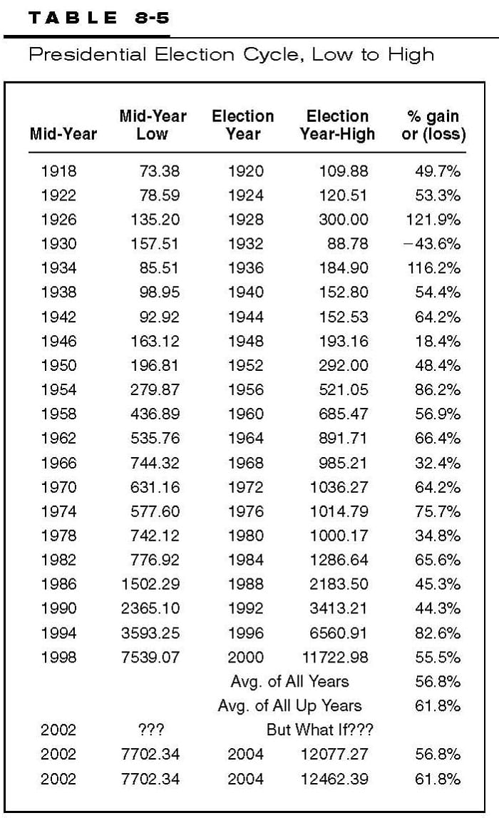
Source: Morning Market Comments, by Don Hays, September 16, 2002. Reprinted with permission of Hays Advisory Group.
The Hays Advisory Group also provided data on the performance of the November through April time frame for each midterm election year from 1950 through 1998.6 Figure 8-1 depicts the S&P 500 Index gains in the midterm (second) election year. As you can see every single year produced a gain. As of July 1, 2003, this midterm election year looks like another winner with the major averages up at least 10 percent for the year to date.
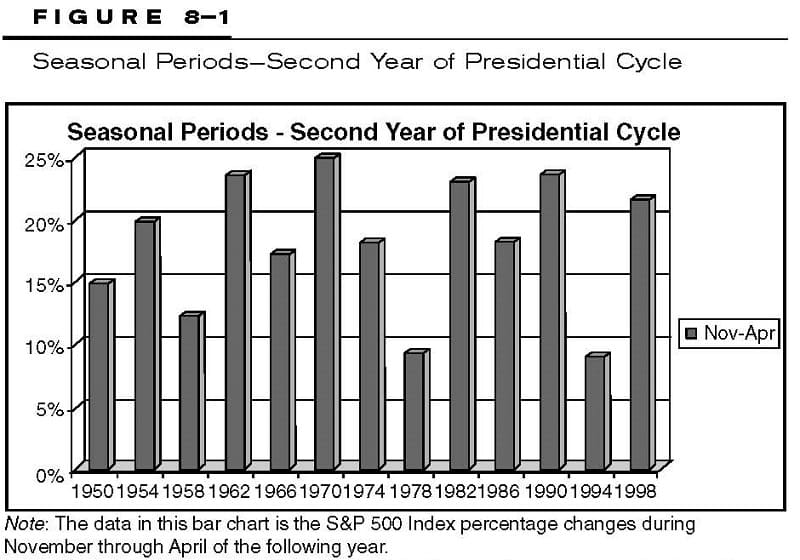
Source: Mark Dodson and Hays Advisory Group. Morning Market Comments, September 26, 2002. Reprinted with permission.
Table 8-6, also provided by the Hays Advisory Group, provides the S&P 500 data not only for the midterm year but the other surrounding years as well.7 Just examining the midterm year November to April performance since 1950, we see that in every instance there was a positive return. The mean return was 18.1 percent, with the lowest return being 9 percent in 1994 and the highest 24.9 percent in 1970. The next best year was the pre-election year with a mean return of 6.3 percent, with only two years of small negative returns.
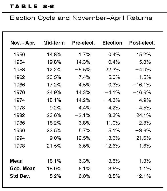
Source: Mark Dodson, and the Hays Advisory Group. Morning Market Comments, September 26, 2002. Reprinted with permission.
The election year November–April period returned an average 3.8 percent with three negative years. Lastly, the postelection year performance was the worst, with a 1.8 percent return with seven down periods.
CONCLUSIONS
Based upon the research by Freeburg, Vakkur, and the Hays Advisory Group, the intelligent investor should carefully consider the potential financial benefits of combining the strongest seasonal monthly and presidential cycle years. By the time you read this book, you will probably have seen the 2003 market peak for the year, and then start its decline again. You may have been in cash for the first half or three-quarters of 2003. Don’t be concerned, since the best six months strategy is coming up around November 1, 2003. And if you miss that time frame, the worst six months period pops up around May 1, 2004. With seasonality investing there is always something happening, either on the long or the short side of the market, and you can invest on both the long and short sides of the market, if you know what you are doing.
Buy-and-hold is certainly not a recommended strategy in any circumstance, especially in light of the ability to use calendar-based investing strategies to limit losses during the weak presidential cycle years—the most recent of which were 2001 and 2002. And true to form those two years provided negative returns to all buy-and-hold investors. The next two weak presidential cycle years are 2005 and 2006, so be prepared for them. The recommended investment vehicles to use for both the seasonal and presidential cycle strategies are index funds, leveraged funds and ETFs (such as the SPY and QQQs). Of course, you will be paying capital gains taxes if you are investing in nonretirement funds, and you won’t be if you are investing your retirement funds. Therefore, these strategies are particularly attractive for your retirement accounts, where your profits compound year over year tax-free.