Trading Articles
Winning Percentage Of A Trading System By Oscar G. Cagigas

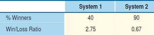
The winning percentage is a critical statistic that can influence the speed at which your capital grows. Find out how you can apply it to your trading system. When developing a trading system, the tendency is to select a particular approach that suits your personality. With this in mind, you can develop a system with a high percentage of winning trades or one with a lower winning percentage, depending on what works best for you. A typical example is a trend-following approach. These systems usually have a winning percentage of 40–50%. Given that it is a system with a good positive expectancy, it doesn’t matter whether this system has a high winning percentage. Developing a system based on expectancy and opportunity is popular. However, the reality is that the winning percentage is a critical statistic that influences the speed at which your capital grows. In this article, I will demonstrate this with a couple of examples.
FROM A KELLY PERSPECTIVE
Suppose we have two different systems. Both have an expectancy of 50 cents per dollar risked. The first system has a winning percentage of 40%; it is a typical trend-following system. The second system has a winning percentage of 90%. It is a typical profit-taking system that takes frequent, small profits. Both systems have the same expectancy equal to $0.50. Using the expectancy formula, we can deduct the win/loss ratio or payoff ratio of the systems. Expectancy can be calculated as:
Expectancy = (1+B)*P-1
where B is the W/L ratio and P is the winning percentage.
System 1 (40% winning trades)
Exp = (1+B) * P – 1
0.5 = (1+B) * 0.40 – 1If you solve for B, you get B = 2.75.
In this typical trend-following system, there is a high win/loss ratio (2.75) and a low winning percentage (40%). Now let’s see what happens with system 2:
System 2 (90% winning trades)
0.5 = (1+B) * 0.90 – 1
Solving for B results in B = 0.67.
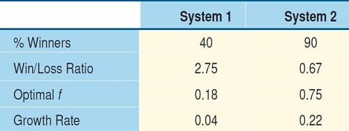
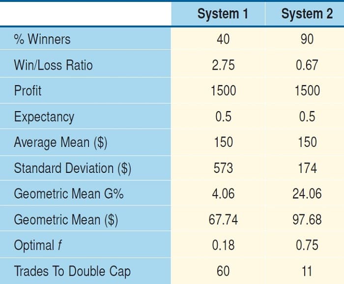
This second system sells when there is a small benefit so there is a low win/loss ratio with a very high winning percentage. So we have two systems with the same expectancy but different characteristics. In Figure 1 we see a summary of the characteristics of these two different systems.
Now, I am going to use the Kelly approach to calculate the optimal fraction to be invested in each system. In doing this, assume a Bernoulli distribution of trades (same amount for all winners, same amount for all losers), which is not the case in trading, but ignore that for a moment to see what happens. The approach allows you to estimate the optimal percentage of your stake to risk in the next trade. As you already know the expectancy, you can calculate the optimal f by dividing the expectancy by the win-loss ratio:
System 1
f = exp/B = 0.5/2.75 = 18%System 2
f = exp/B = 0.5/0.67 = 75%
Although both systems have the same expectancy, the second is clearly better in terms of optimal f. In the first system you should risk 18% of your trading capital in the next trade, while in the second you should risk as much as 75% of your stake in the next trade. If you take that big risk in the second system, it is because you are 90% sure that the next trade is going to be a winner. In the second system, there are only two consecutive losses for every 100 trades, while in the first system there are nine consecutive losses for every 100 trades. This is another advantage of system 2. You don’t need to care about a long string of losses as you would following a trend. In a low winning percentage system, you can go broke as a consequence of a string of losses.
Let’s see how the capital grows. When you risk a fraction of your capital (f%) in a trading system, you produce an exponential growth (exp()) of the equity curve with a factor, which is as follows:
G = p * log(1 + B * f) + (1 – p) * log(1 – f)
where P is the winning percentage, f is the fraction of capital that you risk, and B is the win/loss ratio. The logarithm is natural. G is the exponent of an exponential function (e = 2.71828). The bigger the G, the faster your capital will grow. Again, I am still using the simplification of Bernoulli distribution of trades:
System 1
G = 0.40 * log(1+2.75*0.18) + 0.60 * log(1-0.18) = 0.04System 2
G = 0.90 * log(1+0.67*0.75) + 0.10 * log(1-0.75) = 0.22
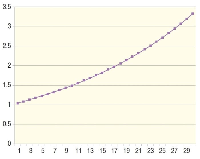
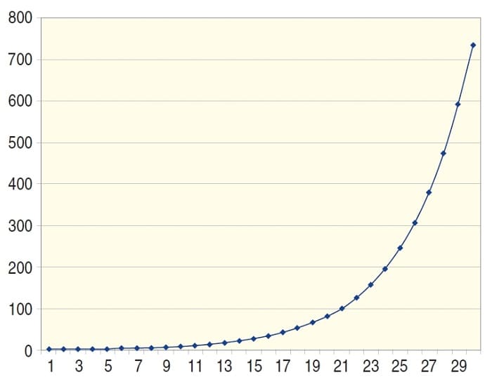
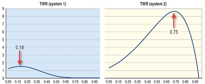
The growth factor is clearly superior in the second system, with 0.22 against 0.04 for system 1 (Figure 2). Figure 3 represents the capital evolution in the first system with a growth factor of 0.04. The capital growth of the second system where G = 0.22 is displayed in Figure 4.
The exponential of G — that is, (2.71828^G) — is the geometric mean of the system. In the first system the geometric mean is 2.71828^0.04 = 1.04, which is 4%. In the second system, the geometric mean is 24.6%. Every time you trade, you are, on average, multiplying by this amount. It is easy to see the significant difference between both systems. When choosing systems with the same expectancy, it is best to go for the one with the best winning percentage, since these kinds of systems will give you faster capital growth. This is logical, since you can expect to be right more often than not. Therefore, you should risk more money accordingly.
TESTING WITH A SEQUENCE OF TRADES
I decided to test the previous results in a more realistic way. Assuming that the distribution of trades is not of the Bernoulli type, I am going to show a sequence of trades that replicates the statistics of the previous example.
System 1 (low winning percentage): This is a set of trades that has a 40% winning percentage and$0.50 of expectancy per dollar risked:
- -300
- -300
- +600
- -300
- +900
- -300
- +1,200
- -300
- -300
- +600
There are 10 trades, four of which are winners (winning percentage = 40%). The win/loss ratio is 2.75, as in the previous example. If I calculate the optimal f and averages of these trades, I find the following (for the calculation, I am using software called SIZER):
- Profit = $1,500
- Expectancy = 0.50
- Win/loss ratio = 2.75
- Optimal f = 0.18
- Arithmetic average trade = $150
- Standard deviation = $573
- Geometric average = 4.06%
- Geometric average trade = $67.74
- If you apply an optimal f strategy (10% diluted) you will duplicate your capital in 60 trades.
System 2 (high winning percentage): This is a set of trades with a 90% winning percentage and$0.50 of expectancy:
- +200
- +200
- -300
- +300
- +400
- +100
- +100
- +200
- +200
- +100
In this case there are 10 trades, nine of which are winners (90% winning).The win/loss ratio is 0.67, as in the previous example. Here are the statistics for this set of trades:
- Profit = $1,500
- Expectancy = 0.50
- Win/loss ratio = 0.67
- Optimal f = 0.74
- Arithmetic average trade = $150
- Standard deviation = $174.6
- Geometric average = 24.06%
- Geometric average trade = $97.68
- If you apply an optimal f strategy (10% diluted), you will duplicate your capital in 11 trades.
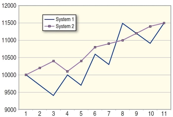
There is a big difference (Figure 5). You are getting $30 more per trade when reinvesting profits in the second system than in the first one (see “Geometric mean $”). Assuming that the trades will continue in the same way, you can expect capital to double in 11 trades with the second system when using a 10% diluted optimal f strategy. You need to make 60 trades to duplicate your capital with the first approach.
In this case, the Kelly approach is accurate and provides almost exact results, although the winning and losing trades don’t have the same dollar value. This is a limited sample of trades and there is a small dispersion. The Kelly formula is less accurate in real trading as the dispersion (standard deviation) of profits and losses increase.
Suggested Books and Courses About Risk Management
The point I need to highlight is that you cannot design a system based on expectancy plus opportunity (number of trades per time unit), since that approach is incomplete. As has been shown here, two systems with the same expectancy will have different equity curves depending on the winning percentage. Moreover, the system with a higher winning percentage will usually have more trades per year, as it has a smaller holding period. The winning percentage will determine the growth rate of the equity of the system (G). The best system in terms of profit is the one with the best geometric mean when traded at the optimal f level, because this system is the one that will generate more profits after reinvestment. Mathematically, the second system in this example is better (Figure 6).
SUMMARY
You have seen how two systems with the same expectancy and final gain can be different. In this example, both systems had the same average gain. They both ended gaining $150 per trade. In the equity curves in Figure 7, you can see that both started with $10,000 and both finished with $11,500. But when you trade with the same risk percentage in both systems, the second appears to be clearly superior. Even if you trade both systems at the optimal risk of the first system (18%), the second system will perform better and have a geometric mean twice the geometric mean of system 1.
The reason for this difference can be attributed to the deviation of the profit & loss data. If the deviation was zero, then the average mean and geometric mean will be the same. But when there is a big deviation of results, the geometric mean reduces its value according to this expression:
Geom = SQRT { am^2 – desv^2 }
where “am” is the average mean and “desv” is the standard deviation of the profit & loss data. SQRT is the square root.
This deviation directly affects the growth of the equity. If you design a trading system only in terms of expectancy (average mean) and opportunity, you are ignoring the fact that another system with the same characteristics will perform better and work better with higher levels of risk if it has a better winning percentage. When there is a low winning percentage, the win/loss ratio is high (usually 2 or more). This difference between the absolute value of winners and losers translates into a higher dispersion.
Both systems had the same maximum loss ($300), but the dollar value of the deviation is three times bigger in system 1. The trend-following approach produces a big dispersion of the results, which affects the equity curve growth.
Oscar G. Cagigas has a degree in telecomunications engineering. He is a private trader with more than 10 years of experience. He is the founder of www.onda4.com, a Spanish-language financial website. He has published three books regarding Elliott wave theory, trading systems, and money management.