Trading Articles
The McGinley Dynamic By Brian Twomey

Apply this market tool devised by a master technician to analyze the forex markets. The McGinley dynamic is a market tool invented by veteran trader/market technician John McGinley. Information about this tool was first published in the Market Technicians Association’s Journal Of Technical Analysis as an outline in 1991 and published there as a full-blown study in 1997. I have attempted here to capture the thought processes of the mind of a master technician as he worked through the process of invention to perfection of this tool. But before that, we must become reacquainted with some staples of technical analysis.
MOVING AVERAGES
A moving average is the study of the history of time series analysis. Early practitioners used various algorithms to smooth data and flatten various-shaped curves, yet this early work was quite primitive. Graduation methods were used later, like a fitting line using a least-squares rule for plotting and construction purposes. Fitting lines using the least-squares rule was later adopted by technical analysis in the family of moving averages. This began the process of interpolating data using probability theories and analysis.
In the Journal Of The Royal Statistical Society in 1909, G.U. Yule described instantaneous averages that R.H. Hooker had calculated in 1901 as moving averages. Yule identified properties of the variate difference correlation method. The term moving averages apparently entered the lexicon shortly after in 1912 through W.I. King’s publication of Elements Of Statistical Methods. Later adopting Yule’s studies, Harold Wold described moving averages in a 1938 study called Analysis Of Time Series. Others attribute exponential smoothing to R.G. Brown’s and Charles Holt’s individual works on inventory control in the 1950s.
EXPONENTIAL SMOOTHING
P.N. Haurlan was the first to use exponential smoothing for tracking stock prices and advanced the study for modern-day technicians. Haurlan referred to “exponential smoothing” as “trend values,” where a 19-day exponential moving average (EMA) was referred to as a 10% trend. His earlier work as a designer of tracking systems for rockets helped him design steering mechanisms. If the steering mechanism was off, it needed further inputs. Haurlan called this “proportional control” and used this method in his groundbreaking studies.
For Haurlan and others, the EMA was the method of choice because of its focus on two inputs as opposed to the simple moving average (SMA) that needed many past datapoints. These early technicians used pure mathematical calculations graphed on chart paper. For example, Haurlan needed a conversion factor, a smoothing constant. His smoothing constant is:
2/(n+1)
where n is the number of days.
So a 19-day EMA equates a 10% trend by 2/(19+1) = 2/20 = 0.10, or a 10% smoothing constant. Proportionate control equals how far price moved from the trend value and adjusts by using trend value curves. This he charted in waves by 1%, 2%, 5%, 10%, 20%, and 50%. Haurlan developed tracking rates based on trends. These tracking rates were measured against a stabilization period. For example, a 50% tracking rate has a five day stabilization period. Technicians Sherman and Marian McClellan added two different EMAs of daily breadth figures, 10% and 5% trend. This gave the first alerts to crossovers when the 10% trend moved above the 5% trend. This detected a market reversal as well as overbought and oversold markets.
The McClellans later invented the McClellan oscillator and the summation index based on their calculations and charting methods during this period. The McClellan oscillator measures the acceleration of daily advance-decline statistics by smoothing with two different EMAs and finding the difference between the two.
Suggested Books and Courses About Market Indicators


Haurlan and Humphrey Lloyd, with Lloyd’s groundbreaking book called The Moving Balance System and his invention of the moving balance indicator, benefited from the easier use of coding EMAs that only needed two inputs: price and the prior value. Back then, computer sophistication wasn’t available, and hence the reason for EMAs over SMAs that needed many datapoints. What separated John McGinley from earlier technicians was his ground-breaking work in moving averages, eventually leading to the McGinley dynamic. What did he see?
There are two problems with moving averages: One, they are inappropriately applied, and two, they are overused.
THE MCGINLEY DYNAMIC: THE EARLY YEARS
According to McGinley, there are two problems with moving averages: One, they are inappropriately applied, and two, they are overused. In addition, they can be outrun by the raw data. Because of this, they should only be applied as smoothing mechanisms, not as trading systems or signal generators. As he said, consider that moving averages range in their uses from fast to slow markets. How can you know which moving averages to use and how to apply them? How can you know when to use a 10-day average rather than a 100-day? Further, moving averages are fixed in length without the ability to change. This is a restriction in their use since they can’t adjust to changing data during trading days. You want to have a smoother that filters the whipsaws, but outliers do exist in averages. What should you do with a 10-day moving average on the ninth or 10th day, considering that much of the trend has been lost?

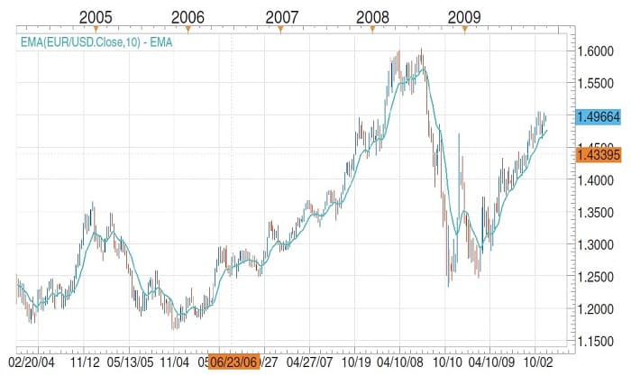
Next, says McGinley, simple moving averages are always out of date. A 10-day average is off by five days or half its length and graphed incorrectly. There is a strong chance that big price moves already occurred within the five days, so the graph set at 10 periods must also be off. An example can be seen in the chart of EUR/USD in Figure 1. The further problem is the dropoff, the difference in price and the line. What if the new data from X days ago is dropped and the data drop is larger than present values? The moving average must also drop, thus generating false signals.
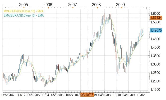
The exponential moving average (EMA) improves on the SMA because calculations allow the average to hug prices more smoothly and allows for faster response to market data. Compare the chart of the EUR/USD in Figure 2 to that of Figure 1. The EMA underperforms in consolidations just as the simple moving average does, generating line breaks and sheer trading indecision.
Exponentials require two inputs, previous average and current price. The classic calculation is A x the previous moving average + B x new data where A + B = 1.0. Usually, a small part of the new data is added to a large piece of the old. To build on Haurlan’s earlier works, for example, an 18% exponential where A = 0.82 and B = 0.18 can be compared to a normal moving average where B = 2/(x+1). So an 18% exponential (x = 10) hugs prices as closely as a 10-day moving average (2/(10+1)) = 18%.
The shape of the exponential may be different due to calculations. The exponential calculation of B can be adjusted to fit market data and prices where SMAs are fixed. It is much more rigid due to its calculations. EMAs therefore follow prices and market changes better than a fixed SMA does. They tend to smooth the data better. See the chart of the EUR/USD in Figure 3. Yet the EMA is not perfect, since adjustments are always needed and it cannot rise with falling prices or fall with rising prices. So what’s the answer?
THE MCGINLEY DYNAMIC
Building on years of moving average research, the McGinley dynamic was invented as a market tool designed to generate less whipsaws, hug prices more closely, adjust calculations to fit the user’s needs, and automatically follow fast and slow markets. Think of the dynamic line of the McGinley dynamic as Haurlan’s steering mechanism, a proportionate control tool that steers the dynamic line along with prices. Does the McGinley dynamic live up to its reputation? Yes. Does it perform the above functions? Absolutely. Building on Lloyd’s work of moving averages where the previous dynamic line was modified, here is the new formula:
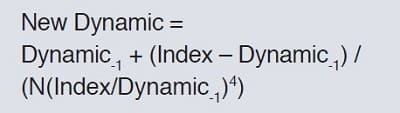
The index may be the Dow Jones Industrial Average (DJIA), the Standard & Poor’s 500, or a stock. McGinley divides the difference between the dynamic and the index by N times the ratio of the two. The numerator gives the up or down sign and the denominator stays within the percentage bounds defined by N. McGinley further states the fourth power, which is the ratio that allows the dynamic line to speed up and follow prices, specifically for down moves. It gives the calculation an adjustment factor that sharply increases the difference between the dynamic line and the current data. He also states that the size of the adjustment changes logarithmically and not linearly. This feature allows the dynamic to hug prices, no matter what the speed of the markets.
McGinley states that N should be 60% of the moving average you wish to emulate. His example is a 20-day moving average that uses an N of 12. The dynamic line adjusts itself by speeding up or slowing down as the market dictates. The second term of the equation is not a factor unless the difference between the index and the dynamic line is large. This aspect of the equation deals with lengths or slopes.
Suggested Books and Courses About Trading Charts


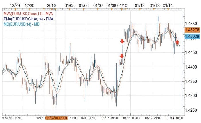
An important factor is the second term, however. McGinley says in fast up markets, the dynamic line slows less than in down markets. It’s the factor of the fourth power that speeds up the dynamic line in down markets. From McGinley’s example, insert 10 for the old dynamic, 5 for the close and N = 7, a product of -6.67. Further, make the close = 14 and you get 0.15. So 14 is far above the old dynamic as 6 is below. This is not a problem, according to McGinley, as the objective is to let profits run and bail out when the market drops. So the upside profits run without whipsaws while the downside adjusts quickly to a drop, allowing opportunity to cut losses. So do you avoid a loss or grab a gain? That’s the decision you need to make. Figure 4 displays the SMA, EMA, and the McGinley dynamic applied again to the EUR/USD currency pair.
WHAT DOES THE MCGINLEY DYNAMIC DO?
John McGinley set out to avoid whipsaws that moving averages are prone to and find a tool that won’t separate prices from the average. The dynamic line rises with falling data. Only one piece of back data is needed. In any trending or trading market, the dynamic doesn’t need backtesting or adjustments. In instances of extreme whipsaw markets, it still sells high and buys low. Moving averages move away from prices and could result in losses, especially when crossovers occur. The McGinley dynamic avoids these dilemmas.
I have used the term “market tool” when referring to the McGinley dynamic. McGinley says the dynamic line is not an indicator and shouldn’t be used as such. He abhors the idea of using the dynamic as a trading vehicle. The McGinley dynamic is not only a remarkable tool, but it is the product of many years of intense research and insight by a master technician.
Brian Twomey is a currency trader and adjunct professor of Political Science at Gardner-Webb University. He would like to thank John McGinley for bringing forth the dynamic. Twomey also thanks Tom McClellan, editor of the McClellan Market Report, for access to research. And finally, giant thank yous to Jeanette Young, the “option queen” at the Market Technicians Association, for her help.