Trading Articles
Price-Time Radius Vector (PTV): Geometric Market Timing Method
A variety of techniques attempt to forecast prices in financial markets. However, relatively few deal with the most important element in financial market timing, i.e., time. Traditional cycle analysis is the most commonly used of these techniques, but even the so-called experts on this subject acknowledge the great limitations of their approach. Cycles (or more correctly, rhythms) tend to suddenly disappear, only to reappear at a later date with phase shifts from their original pattern. Contemporary cycle analysts cannot explain why cycles “disappear”, why they reappear with a phase shift, and a variety of other characteristics that will be explained in this course.
DEFINITION OF THE PRICE-TIME RADIUS VECTOR (PTV)
To begin the analysis of the dimension of time it must be understood that financial market movements are defined within the limits of radii vectors. These vectors allow analysts to expand their thinking beyond one dimension at a time, i.e., only price levels or only time values, and to START VIEWING PRICE-TIME AS A SINGLE UNIFIED ELEMENT. For, as will be shown in this course, PRICE AND TIME ARE INTIMATELY CONNECTED.
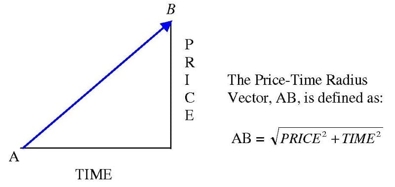
On a traditional price-time chart of any financial market, the price-time radius vector is defined as shown in Figure 1.1. For the sake of brevity, the price-time radius vector will, hereafter, be referred to as PTV. This is an application of the Pythagorean theorem taught in high school geometry classes, which states that the sum of the squares of the sides of a right triangle is equal to the square of the hypotenuse. In this case, the sides of the right triangle are time and price, and the hypotenuse is the PTV.
- THE PTV HAS CONSTANT LENGTH AND DEFINES THE INTERVAL OF OPERATION WITHIN SPECIFIED MARKET CONDITIONS.
CALCULATION OF THE PTV
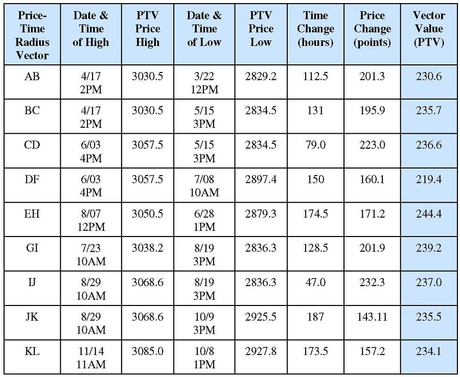
Chart I.A is used to demonstrate how the PTV is calculated. On this price-time chart the time distance between the two points labeled B and C was 131 trading hours.3 The price change between these same two points was 195.9 points. Therefore, using the equation from Figure 1.1, the PTV, BC, is calculated to be the square root of (1312 + 195.92), which equals 235.7. This technique is repeated for each of the PTVs shown on Chart I.A, and the results are contained in Table 1.1.
Tables similar to Table 1.1 will be used throughout Part I of this course. They contain the data used to calculate all PTVs. It is highly recommended the reader reference Appendix E at this point to avoid any possible confusion about how the data used in this course is collected or calculated. If the reader is not interested in verifying the data used to calculate the PTVs, then the only necessary part of these tables is the last column, which contains the final values of the PTVs. For example, in Table 1.1 the first row of data shows the PTV, AB, to equal 230.6.
When the PTV values from column eight of Table 1.1 are studied, one of the first things noticed is that they are all approximately the same length. The only deviation occurred at the bottom labeled F (radius vector DF = 219.4), which was caused by the overlapping radius vector EH. On Chart I.A note that F lies on the line connecting E and H.
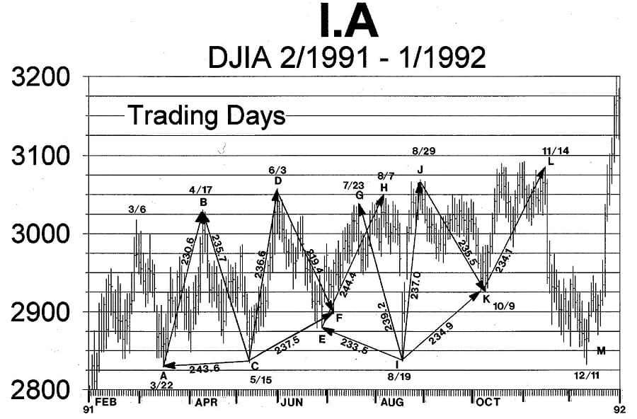
One reason why market analysts have failed to notice that all these market movements were equal in length is that the scales of the price and time axes must be just right in order for this phenomenon to be immediately visible on a price-time chart. Specifically, the price axis must reflect one unit of price for each unit of time.4 As the scales deviate from this one-to-one relationship the appearance of the vectors will be more and more distorted from their actual size. To make this clearer, refer again to Chart I.A. Notice that radius vector CD appears to be longer than radius vector CF. However, calculations have proven they are equal in length. The distortion is caused because Chart I.A is not “squared out”. If the time scale of this chart was stretched out these vectors would appear to be closer in length. Regardless of the scales used for the two axes on a chart, by employing the technique described above the actual length of the radius vector is determined, and the graphical approach is unnecessary.
PTVs ROTATE AROUND A COMMON CENTER
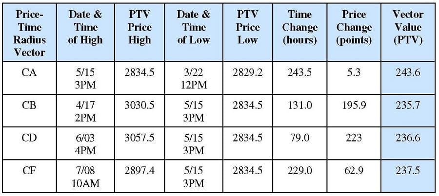
On Chart I.A the points “C” and “I” hold special significance. These two points represent the center points about which these two radii vectors rotate in a clockwise direction. The “C” radius vector starts with CA, sweeps through CB, over to CD, and finally terminates with CF. The “I” radius vector starts with IE, sweeps through IG, over to IJ, and finally terminates with IK.
An interesting concept is that these two rotating radii vectors have their beginning points defined before their center points have been reached in time. For example, at point A the radius vector swinging from A to B is already moving within the limits of the radius vector centered at point C, EVEN THOUGH POINT C HAD YET TO OCCUR IN TIME. The following radii vectors are equal length:
- CA = 243.6
- CB = 235.7
- CD = 236.6
- CF = 237.5
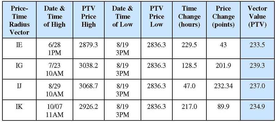
The values used for the calculation of these radii vectors are contained within Table 1.2. Similarly, Table 1.3 shows that the radii vectors rotating around point “I” have equal lengths:
- IE =233.5
- IG = 239.3
- IJ =237.0
- IK = 234.9
The reason why radius vector DF was shorter than the other vectors is now apparent. The sequence of radii vectors rotating around point C terminated with radius vector CF. However, the radii vectors rotating around point I began with radius vector IE. This means the two cycles overlapped by the amount EF, causing the terminal point of DF to be “pulled up” by the radius vector rotating around point I.
THE PTV ANGLE DEFINES THE EXTENT AND DURATION OF A MOVE
Since the length of the PTV is constant, it follows that as the time component decreases the price component increases, and vice-versa. By knowing the length of the radius vector the analyst is able to project the magnitude and DURATION of a move. If a fast advance is under way he knows it will not last very long. Similarly, a slowly advancing market will show little price gain because the length of the radius vector will be consumed by the component of time, leaving little for price.
Advanced Books and Courses on Market Cycles & Timings


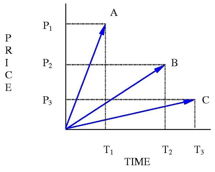
In Figure 1.2 the PTVs OA, OB, and OC are all equal length. OA advanced very quickly to its maximum length, i.e., T1 is a very short time interval; consequently, the price component of OA, P1, is very large. As the angle between the PTV and the time axis decreases, the time component increases and the price component decreases. That is, the time component of OB, T2, is longer than the time component of OA, T1. And the price component of OB, P2, is less than the price component of OA, P1.
Similarly, as the angle becomes even flatter with the time axis, as with OC, the time component, T3, becomes greater than that of either OA or OB. And the price component of OC becomes less than that of either OA or OB.
A real-life example of a PTV similar to OA is shown on Chart I.A between points C and D. The time component of CD was short, only 79 hours. Hence, its price component must be long in order to maintain a constant length radius vector. In fact, the price component of CD was 223 points, which approaches the maximum amount for a PTV at this energy level.
An example of a PTV similar to OB is shown on Chart I.A, between points E and H. Between those two points the time component was 174.5 hours. Hence, the price component must be shorter than it was in CD to maintain the constant length radius vector. In fact, the price component was 171.2 points.
PTV AND THE MUSICAL SCALE
The frequency of notes on the musical scale are defined by ratios of simple integers relative to the fundamental tone (such as the octave=2:1, the fifth=3:2, the fourth=4:3, etc). Similarly, lengths of PTVs are defined by the same ratios as found on the musical scale.
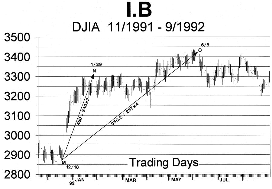
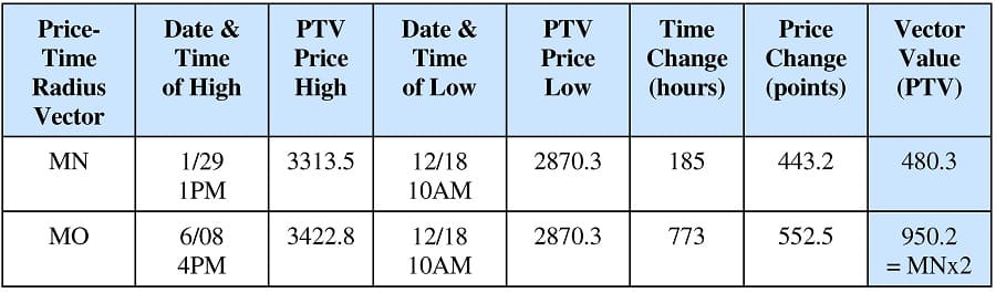
For example, Chart I.B (Table 1.4) is a continuation of Chart I.A. On Chart I.B, between points M and N, the time distance was 185 hours and the price component was 443.2 points. Using the technique described above, the PTV between points M and N (hereafter, referred to as MN) is calculated to be 480.3, which is two times (the octave) the amount calculated for the radii vectors on Chart I.A. The octave above PTV, MN, can be seen on Chart I.B, between points M and O (hereafter, referred to as MO) where the time component was 773 hours and the price component was 552.5 points. Hence, the PTV, MO, is calculated to be 950.2, which is twice (the octave) the length of MN and four times (the double octave) the radii vectors shown on Chart I.A.
PTVs CAN EXTEND FOR CENTURIES
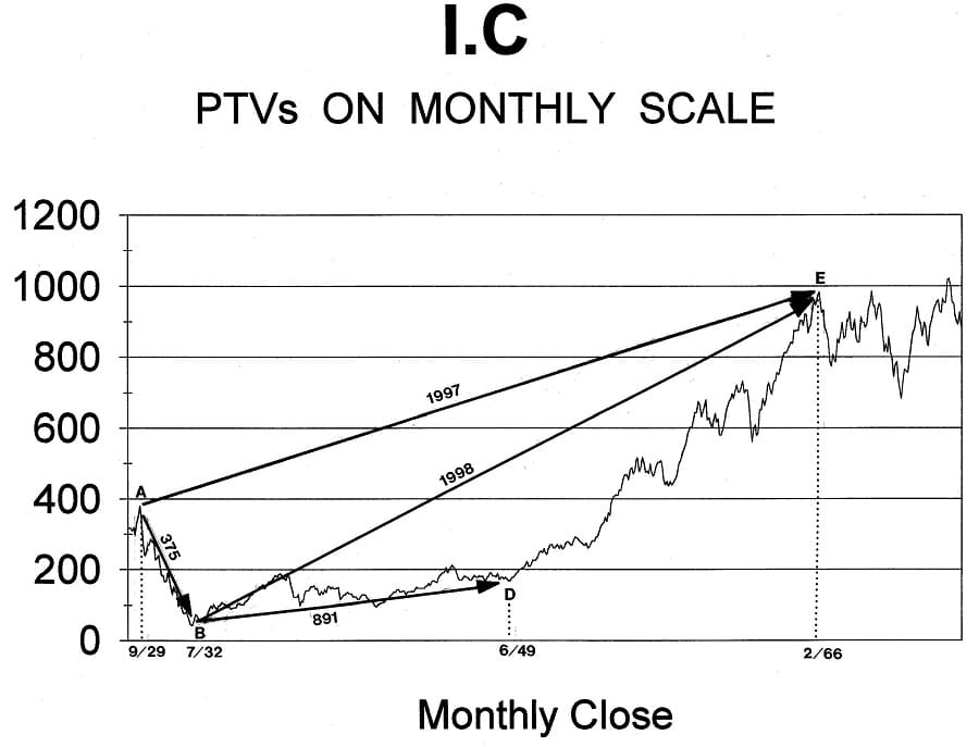
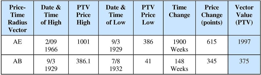
Application of the PTV is not limited to daily charts. In fact, there is no limit to how large (or small) a PTV can be. For example, Chart I.C is a chart of the stock market from 1929 to 1966, where the PTV, AE, is calculated using weekly data to be 1997 price-time units in length. The values used for this calculation are shown in Table 1.5. This PTV will be used in later lessons to show the geometric structure during this time period.