Trading Articles
Intraday vs Overnight Returns: Erik Skyba’s Statistical Study
Anomalies in the markets appear on occasion and challenge the efficient market hypothesis. Here’s a look at the overnight return anomaly, with some findings that may surprise you. Many within the financial community believe that the markets follow the efficient market hypothesis. This theory asserts that the current price of a security reflects all public and private information about that security. Changes in price are due to current news or events, which are impossible to predict. Thus, a tradable follows the path of a random walk, the premise of which states that current prices are not dependent on past prices and are normally distributed over time.
Over the years, many studies have presented data about what academics call “market anomalies.” These anomalies appear from time to time and challenge the efficient market hypothesis. There are three common classifications: fundamental, technical, and calendar-based. There is another class of anomaly that most people simply refer to as “other” for those that do not fit into the original three. In this article we will discuss one of these “other” market anomalies, called the overnight return.
Overnight Return Anomaly Rules:
Buy at the close of the day session
⇒ Hold position overnight
Sell at the open of the next day’s session
CAN YOU MAKE RETURNS OVERNIGHT?
Day versus overnight returns can be studied by analyzing the differences in returns between the day’s session (defined here as regular NYSE trading hours) and the overnight period. In testing the returns for the day and overnight periods, we used the SPDR S&P 500 exchange traded fund (SPY) from February 2, 1993 to June 7, 2010. We can define the day’s return as the difference between the day’s open and the day’s close. The overnight return is the difference between the day’s close and the following morning’s open.
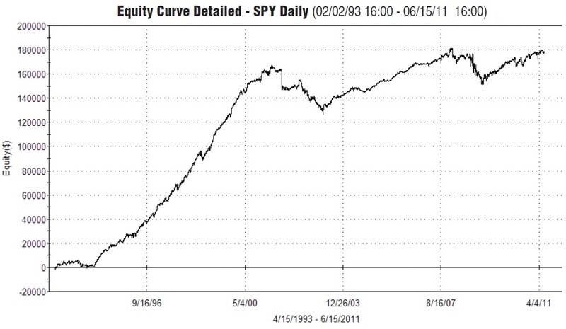
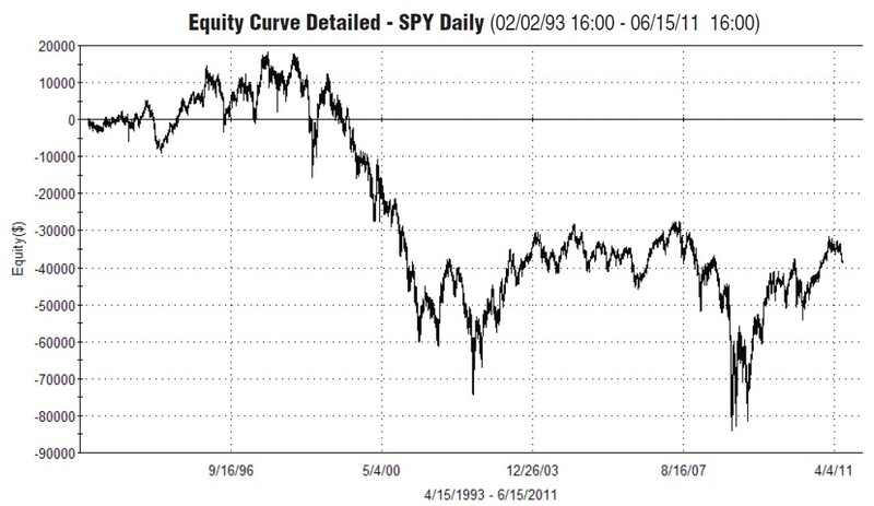
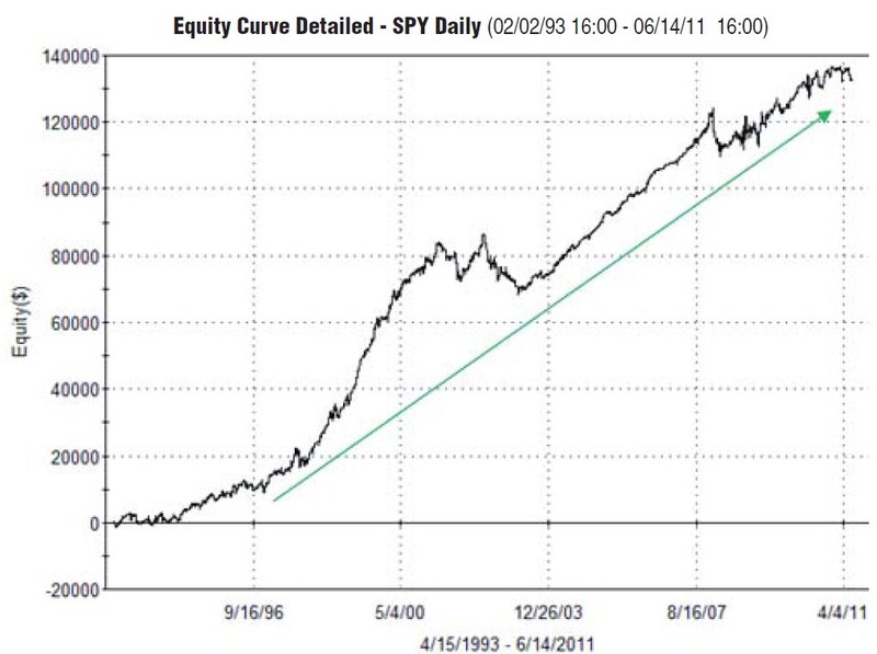
It is a common misconception on the part of most market participants that the majority of returns from day-to-day trading are extracted from the daytime period, rather than from the overnight. This would make sense, as more people track the daytime price action as opposed to the overnight price action. But as Figures 1 and 2 indicate, the opposite is true of day versus overnight returns.
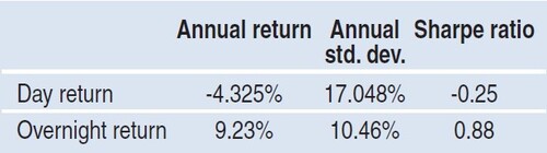
In Figure 3, we note that SPY has an annual overnight return of 9.23%, while the daytime return is -4.325%. Also of interest are the annual standard deviation values, which are lower during the overnight period than during the daytime action. Not only does this raise the possibility of a greater return in holding a position overnight, but it may also be less risky to do so, which is why the Sharpe ratio (which does not include the risk-free interest rate in our calculation) for the overnight period is 0.88 compared to the Sharpe ratio during the daytime period, which is -0.25.
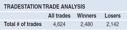
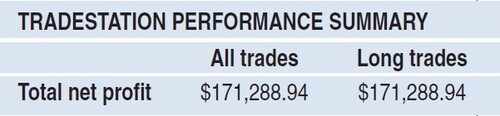
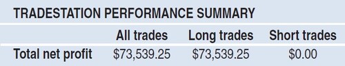
The main issue with these results as they relate to the overnight return is that over time there are too many trades that, on average, do not produce enough profit to overcome commission costs. We can see from Figure 4 that the backtest generated 4,624 trades. Commission costs of $0.01 per share caused our net profit to decrease from $171,288.94 to $73,539, as shown in Figures 5 and 6. However, if we were to make the commission cost $0.02 per share or we were to add slippage costs, the total net profit of the overnight return would be less than zero.
SPECIFIC TIME PERIODS
Perhaps the actual overnight return can be identified as specific deviation values low, as the results in Figure 3 indicate. Further analysis of overnight return distributions may be conducted to determine the specific time period where these returns originate. Exchange traded funds (ETFs) trade pre- and post-market hours, which make up a portion of what we have defined as the overnight period. The hours we are examining are from 4:00 pm to 8:00 pm Eastern time (ET) for the post-market session and 6:00 am to 9:30 am ET for the premarket session. The day’s session, also known as the regular session, is from 9:30 am to 4:00 pm ET. Recall that our overnight return study included daily data as far back as February 2, 1993. For this additional study, we surveyed data going back to November 1, 2002.
Advanced Books and Courses on Algorithmic & Quant Trading


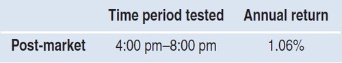
Two observations will provide further insight into how the overnight return is achieved. First of all, premarket returns are greater than post-market returns. The average annual return for the SPYs in the post-market period (4:00 pm to 8:00 pm) was 1.06% (Figure 7), while premarket returns (6:00 am to 9:30 am) averaged 3.37% (Figure 8).
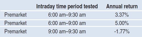
For reasons unknown, the market appears to be bid up more in the premarket session than in the post-market. In addition, from 9:00 am to 9:30 am, the market on average is lower, with an annual return of -1.77% (Figure 8). Perhaps the most impressive observation is that the market returned 5.00% (Figure 8) annually from 6:00 am to 9:00 am, omitting the 30 minutes of trading before the regular session opens. Figure 8 depicts a detailed investigation of premarket trading returns for SPY.
CLOSE RELATIVE TO PREVIOUS DAY
There are also differences in the overnight return performance when the daytime session has a higher or lower close than that of the previous day. In Figures 9 and 10, we see that the overall performance in the overnight period was better when today’s close was less than yesterday’s.
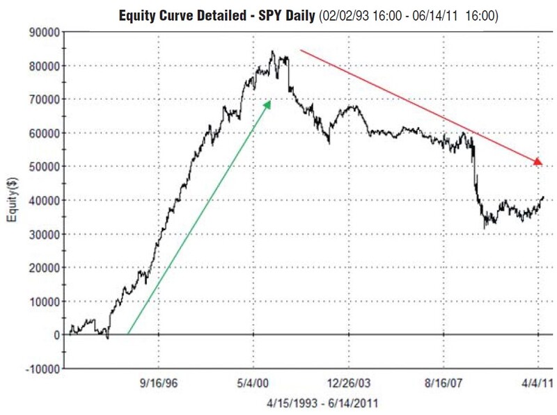
Although both equity curves did well from 1993 to 2001, since 2001 there has been noticeable outperformance in the overnight return when the day’s close is less than the previous day’s close (Figure 10).
CONSISTENT RESULTS ACROSS ETFS
Surprisingly, the overnight return anomaly is remarkably consistent. It exists in many of the S&P iShare ETF sectors and style boxes we analyzed. Most of these ETFs are composed of large-capitalization stocks, with the exception of the Russell 2000 iShare ETF and the S&P MidCap 400 ETF. We ran our study on the entire life of 12 ETFs, the results of which can be seen in Figure 11.
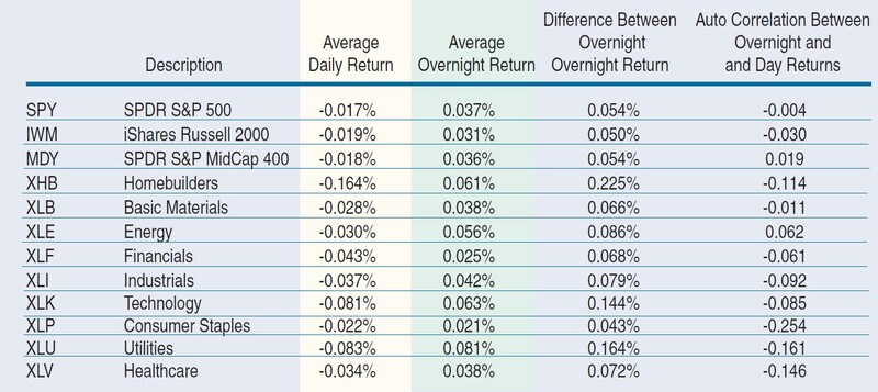
For each ETF, we can see the average overnight return significantly differs from the average daytime return. For the 12 ETFs we examined, we found a higher average return in the overnight period than we did in the daytime session, with the most notable differences being in the utilities, technology, energy, industrials, and homebuilders sectors. (Homebuilders had the shortest data history available in February 6, 2006, to January 1, 2011.) The technology, utility, and homebuilding sectors showed the largest differentials in returns at 0.144%, 0.164%, and 0.225%, respectively.
Another finding from our study was that the autocorrelation values between the average overnight return and the average daytime return were negative. Autocorrelation is a mathematical calculation that is typically used to compare the time series today with a lagged time series n periods in the past. The purpose is to see what degree of trending bias exists in the data. It is telling us the level of correlation the overnight return has with the daytime return. The values for autocorrelation range from -1 to +1, with the value of +1 a highly correlated positive relationship in which both returns are moving in the same direction. A value of -1 means that there is an inverse relationship in which the returns move in completely opposite directions.
When we analyze the autocorrelations data from Figure 11, we see that the values are negative for almost all symbols except the SPDR S&P MidCap 400 (MDY) and SPDR S&P Energy (XLE). The highest levels of negative autocorrelations are in the consumer staples, health care, and utilities sectors.
Two important points must be emphasized about the findings in the autocorrelation values. First, keep in mind what most active traders “believe” — that trading is emotional and if the day’s return is positive or negative, most traders would expect follow-through into either the overnight period or the next day’s session. If the day’s return is positive, then that return will translate into a positive overnight session or vice versa. The higher or lower the day’s returns are, the expectations are greater for a positive or negative follow-through session.
BUT THAT MAY NOT BE THE CASE
Our study shows the opposite behavior. For the most part, we found autocorrelation values to be negative, which means that there is no value in thinking that if the day’s return is positive, then this will translate into a positive return for the overnight session. You may already have inferred this information from the equity curves in Figures 1 and 2. Because the autocorrelations are negative, it may be better to do the opposite or, at the very least, incorporate this information into your daily trading plans as a bias.
While these autocorrelations are statistically significant from what would be considered random values, the usefulness of this information for strategy developers will depend on their ability to incorporate these biases into a meaningful trading system.
- Erik Skyba is a senior quantitative analyst for TradeStation and is a Chartered Market Technician.